GMT topography colours (I)
Jan 30, 2014
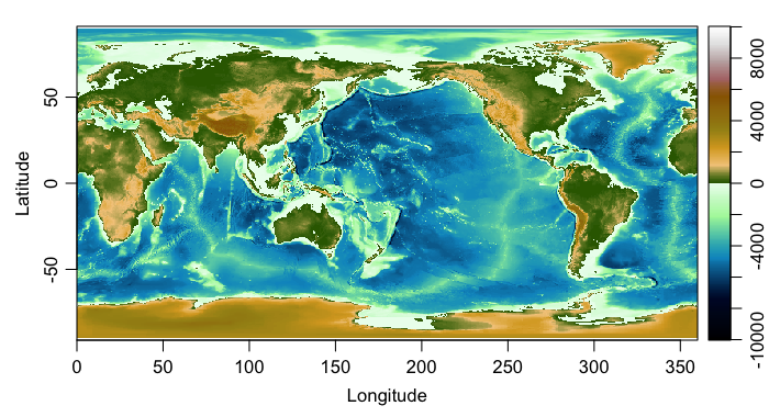
The GMT colour palette is illustrated with ocean topography.
I enjoyed the blog posting by “me nugget”, which I ran across on R-bloggers, and so I decided to try that author’s GMT colourscheme. This revealed some intriguing patterns in the Oce dataset named topoWorld. The following code produces a graph to illustrate.
1. Set up colours as suggested on the “menuggest” blog
1
2
3
4
5
6
7
8
9
10
11
## test GMT colours as suggested by
## http://menugget.blogspot.ca/2014/01/importing-bathymetry-and-coastline-data.html
ocean.pal <- colorRampPalette(c("#000000","#000209","#000413","#00061E",
                                "#000728","#000932","#002650","#00426E",
                                "#005E8C","#007AAA","#0096C8","#22A9C2",
                                "#45BCBB","#67CFB5","#8AE2AE","#ACF6A8",
                                "#BCF8B9","#CBF9CA","#DBFBDC","#EBFDED"))
land.pal <- colorRampPalette(c("#336600","#F3CA89","#D9A627","#A49019",
                               "#9F7B0D","#996600","#B27676","#C2B0B0",
                               "#E5E5E5","#FFFFFF"))
library(oce)
## Loading required package: methods
## Loading required package: mapproj
## Loading required package: maps
1
2
3
4
5
6
data(topoWorld)
waterBreaks <- seq(-10000, -100, by=50)
landBreaks <- seq(100, 10000, by=50)
imagep(topoWorld, asp=1,
breaks=c(waterBreaks, 0, landBreaks),
col=c(ocean.pal(length(waterBreaks)), land.pal(length(landBreaks))))
Resources
- Source code: 2014-01-30-gmt-colors-topography.R