Introduction
I was watching a video of David Suzuki being interviewed on Australian TV, and
there were some questions about the “pause” in temperature in the GISS dataset.
I thought I’d like to check for myself, and reasoned that I may as well update
the giss dataset in the ocedata R package.
As always seems to be the case, the data format is changed a bit from autumn
2014, when I downloaded GISS and put it into ocedata, so I had to write
some new code.
I also found a data file on my machine that I downloaded some time in the past,
but my tests tell me that it is not the one I used for ocedata. Thus, I
have three datasets to explore.
At the risk of providing fuel for debate about such things, I am presenting code and graphs that show what I found. I make no claims to accurate processing. For one thing, the only file for which I have a clear download history is the one dated today [3].
Procedure and results
First, I downloaded the latest dataset from [1], storing it in a file named
giss-2015-11-07.dat (provided in [3] here). Then I found another file,
evidently from 2014, which I copied locally and renamed giss-2014-xx-xx.dat
([4] here). Note that the file formats differ slightly, in the asterisks near
the end; the new format has spaces, which make it easier to read the data,
whereas the old format is clearly designed for fixed-width data readers.
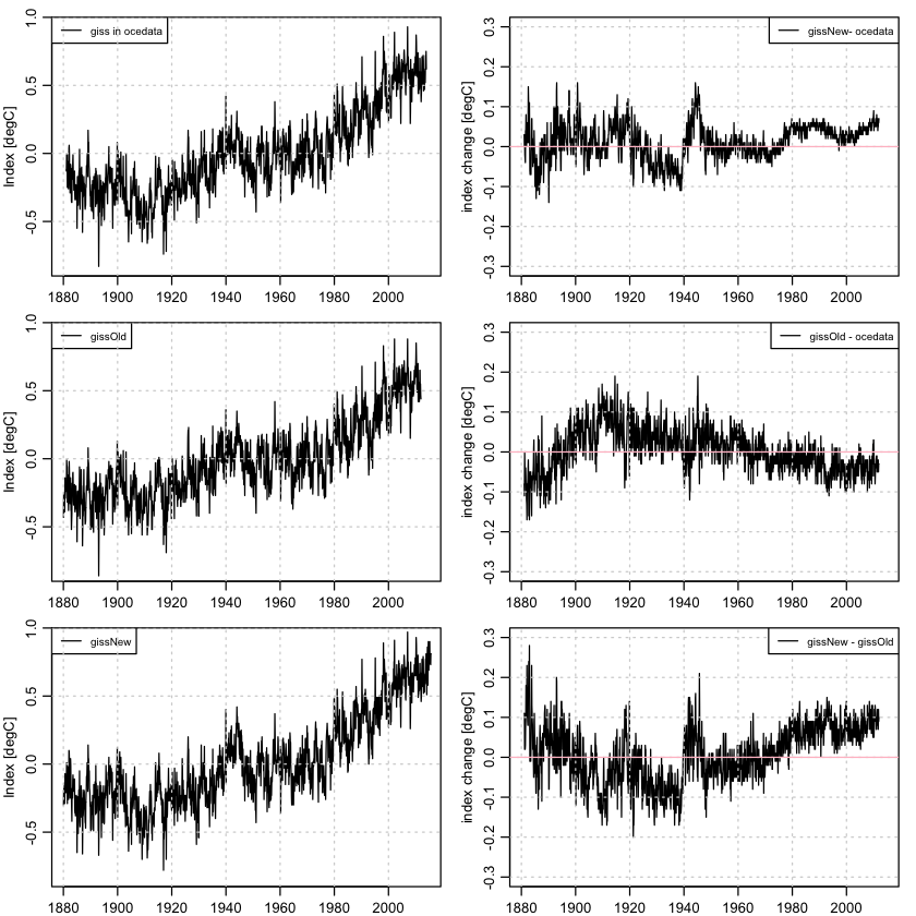
Then I wrote code to read the new file. Then I plotted timeseries (left column) and some differences (right column).
My code is ugly and ad-hoc. It may contain errors, and the main reason I’m posting this is to invite readers to email me if they see any errors. (Comments are turned off because I don’t have time to moderate them, and unmoderated comments on a blog that might touch on climate issues is a bit like dropping a lit match over a pool of gasoline and hoping for the best.)
1
2
3
4
5
6
7
8
9
10
11
12
13
14
15
16
17
18
19
20
21
22
23
24
25
26
27
28
29
30
31
32
33
34
35
36
37
38
39
40
41
readGISS <- function(file)
{
    lines <- readLines(file)
    yearLine <- grep("Year", lines)
    l <- lines[seq.int(head(yearLine,1)+1, tail(yearLine,1)-1)]
    l <- l[grep("Year", l, invert=TRUE)]
    l <- l[grep("^$", l, invert=TRUE)]
    l <- gsub("\\*+", "  NA", l)
    d <- read.table(text=l)
    yearorig <- d$V1
    months <- cbind(d$V2, d$V3, d$V4, d$V5,
                    d$V6, d$V7, d$V8, d$V9,
                    d$V10, d$V11, d$V12, d$V13)
    index <- as.vector(t(months)) / 100
    ## the 1/24 centres in months (at least roughly)
    year <- seq(yearorig[1], length.out=length(index), by=1/12) + 1/24
    keep <- !is.na(index)
    data.frame(year[keep], index[keep])
}
readGISS2014 <- function(file)
{
    l <- readLines(file) # http://data.giss.nasa.gov/gistemp/tabledata_v3/GLB.Ts+dSST.txt
    l <- l[grep("^[1-2].*", l)]            # ignore headers at start, and every 20 years
    ## year is in char 1 to 4; data in 0.01degC are in char 8 to 65
    startyear <- scan(textConnection(l[1]), n=1)
    l <- substr(l, 8, 65)
    l <- l[grep("\\*+", l, invert=TRUE)]    # ignore lines with missing month data
    index <- 0.01 * scan(textConnection(l))
    year <- 1/24 + seq(startyear, by=1/12, length.out=length(index))
    data.frame(year=year, index=index)
}

## Read two text file, then load data(giss, package="ocedata") prior to 2015-11-16
gissNew <- readGISS("giss-20151107.dat") # see [3] below
gissOld <- readGISS2014("giss-2014xxxx.dat") # see [4] below
load("giss-ocedata-until-20151116.rda") # yields 'giss'; see [5] below
## print some tests; note that we offset gissOld by 1 year because
## readGISS2014() skips any year with missing data (including the
## first year, which has a missing season) ... this function is just
## a kludge for this blog item, so don't worry about this!
print(giss$index[1:12])
##  [1] -0.12 -0.13 -0.01 -0.01 -0.01 -0.25 -0.10 -0.06 -0.16 -0.21 -0.26
## [12] -0.17
1
print(gissOld$index[13:24])
##  [1] -0.20 -0.24 -0.01 -0.05 -0.06 -0.32 -0.14 -0.12 -0.26 -0.29 -0.38
## [12] -0.30
1
2
3
4
5
6
7
8
9
10
11
12
13
14
15
16
17
18
19
20
21
22
23
24
25
26
27
28
29
30
31
32
33
34
35
36
37
38
39
par(mar=c(1.7, 3, 1, 1), mgp=c(2, 0.7, 0), mfcol=c(3, 2))
plot(giss$year, giss$index, type='l', ylab="Index [degC]")
legend("topleft", lwd=1, legend=c("giss in ocedata"), bg="white", cex=3/4)
grid()
## store the scale
xlim <- range(giss$year)
ylim <- range(giss$index)
plot(gissOld$year, gissOld$index, type='l', ylab="Index [degC]", xlim=xlim, ylim=ylim)
legend("topleft", lwd=1, legend=c("gissOld"), bg="white", cex=3/4)
grid()
plot(gissNew$year, gissNew$index, type='l', ylab="Index [degC]", xlim=xlim, ylim=ylim)
legend("topleft", lwd=1, legend=c("gissNew"), bg="white", cex=3/4)
grid()
start <- max(c(min(giss$year),min(gissOld$year),min(gissNew$year)))
end <- min(c(max(giss$year),max(gissOld$year),max(gissNew$year)))
look <- start<=giss$year&giss$year<=end
lookOld <- start<=gissOld$year&gissOld$year<=end
lookNew <- start<=gissNew$year&gissNew$year<=end
plot(gissNew$year[lookNew], gissNew$index[lookNew]-giss$index[look],
type='l', ylab="index change [degC]", xlim=xlim, ylim=c(-0.3, 0.3))
grid()
abline(h=0, col='pink')
legend("topright", lwd=1, legend=c("gissNew- ocedata"), bg="white", cex=3/4)
plot(gissOld$year[lookOld], gissOld$index[lookOld]-giss$index[look],
type='l', ylab="index change [degC]", xlim=xlim, ylim=c(-0.3, 0.3))
grid()
abline(h=0, col='pink')
legend("topright", lwd=1, legend=c("gissOld - ocedata"), bg="white", cex=3/4)
plot(gissOld$year[lookOld], gissNew$index[lookNew]-gissOld$index[lookOld],
type='l', ylab="index change [degC]", xlim=xlim, ylim=c(-0.3, 0.3))
grid()
abline(h=0, col='pink')
legend("topright", lwd=1, legend=c("gissNew - gissOld"), bg="white", cex=3/4)
Conclusions
The three datasets differ. Having taken poor notes on the two earlier ones, I cannot say for sure when they were downloaded, although the headers in these files are quite informative.
One might prefer newer datasets to older ones, since (a) they contain new
observations and (b) they presumably have more accurate old data, given ongoing
work to improve analysis methods and data selection. For that reason, the next
update of ocedata will use whatever version of GISS is available at the
time of packaging.
Readers interested in recent changes to GISS (and this includes me!) might do well to start their reading with the NASA summary of changes [2].
References and resources
-
Jekyll source code for this blog entry: 2015-11-07-giss.Rmd