Introduction
The motivation and methodology was discusssed in Part I [2] and so here I will just give code and resulting diagrams, and then make some tentative conclusions. Importantly, the present analysis revises the two Halifax examples, and adds a well-studied case for the Three Sisters peaks in the Oregon Cascades [1].
1
2
3
4
5
6
7
8
9
10
11
12
13
14
15
16
17
18
19
20
21
22
23
24
25
26
27
28
29
30
31
32
33
34
35
36
37
38
39
40
41
42
43
44
45
46
47
48
49
50
51
52
53
54
55
56
57
library(oce)
if (0 == length(ls(pattern="^d$")))
    d <- read.landsat("/data/archive/landsat/LC80450292013225LGN00")

## http://earthobservatory.nasa.gov/blogs/elegantfigures/2013/10/22/how-to-make-a-true-color-landsat-8-image/

L <- c(0.24, 0.12)
threeSisters <- c(-121.73, 44.13)
ts <- landsatTrim(d, ll=threeSisters-L, ur=threeSisters+L)

demo <- function(l, red.f, green.f, blue.f, offset=rep(0,4), name=NULL, label="")
{
    dim <- dim(l[["red"]])
    w <- 6
    h <- round(w * dim[2] / dim[1], 2) # proper ratios can yield horiz. stripes
    if (!is.null(name))
        png(name, unit="in", width=w, height=h, res=100, pointsize=9)
    plot(l, band="terralook", mar=c(2, 2, 1.5, 1),
         red.f=red.f, green.f=green.f, blue.f=blue.f, offset=offset)
    mtext(label, font=2, side=3, line=0, adj=1)
    mtext(sprintf("red.f=%g green.f=%g blue.f=%g offset=c(%g,%g,%g,%g)",
                  red.f, green.f, blue.f, offset[1], offset[2], offset[3], offset[4]),
          side=3, line=0, adj=0)
    if (!is.null(name)) dev.off()
}

## red.f, green.f and blue.f as in posting from yesterday
demo(ts, 1.7, 1.6, 6, rep(0,4), "2016-02-21-landsat-01.png", "Fig. 1A")

## Reducing blue factor removes the blue tinge to the land,
## at the expense of making the clouds unnaturally green. Also,
## various land areas are still not as red as in the reference
## image.
demo(ts, 1.7, 1.6, 3, rep(0,4), "2016-02-21-landsat-02.png", "Fig. 1B")

## After some adjustment of red, green and blue together, the results can
## be improved to some extent.
demo(ts, 2.2, 1.6, 5, rep(0,4), "2016-02-21-landsat-03.png", "Fig. 1C")

## Next, try altering the offset in the linear relationship,
## as opposed to the multiplicative factor. This is done with
## the `offset` argument, rather than with `red.f`, etc.
demo(ts, 1.7, 1.5, 6, c(0,-0.05,-0.2,0), "2016-02-21-landsat-04.png", "Fig. 1D")

## For reference, apply these values to the Halifax
## winter test image.
load("Hw.rda")
demo(Hw, 1.7, 1.6, 6, rep(0,4), "2016-02-21-landsat-05.png", "Fig. 2A")
demo(Hw, 1.7, 1.6, 2, rep(0,4), "2016-02-21-landsat-06.png", "Fig. 2B")
demo(Hw, 2.2, 1.6, 5, rep(0,4), "2016-02-21-landsat-07.png", "Fig. 2C")
demo(Hw, 1.7, 1.5, 6, c(0,-0.05,-0.2,0), "2016-02-21-landsat-08.png", "Fig. 2D")

load("Hs.rda")
demo(Hs, 1.7, 1.6, 6, rep(0,4), "2016-02-21-landsat-09.png", "Fig. 3A")
demo(Hs, 1.7, 1.6, 2, rep(0,4), "2016-02-21-landsat-10.png", "Fig. 3B")
demo(Hs, 2.2, 1.6, 5, rep(0,4), "2016-02-21-landsat-11.png", "Fig. 3C")
demo(Hs, 1.7, 1.5, 6, c(0,-0.05,-0.2,0), "2016-02-21-landsat-12.png", "Fig. 3D")
Results and discussion
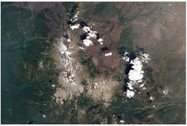
First, here is the reference image from [1], as adjusted in great detail, using more sophisticated methods than are presently available in oce.
Now, below are the results from the 4 trials for this image. Refer to the code
above for methodology, but note that the line at the top of each image
summaries the relevant arguments to plot.landsat().
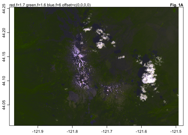
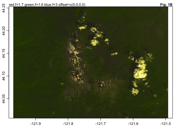
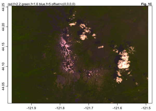
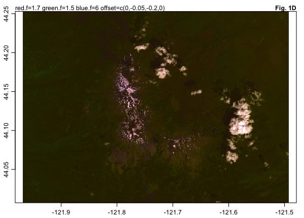
The blueness of the land in Fig 1A is alleviated in Fig 1B, although at the expense of an overall green tinge. Increasing the red factor, as in Fig 1C, improves the land colour somewhat, but I found it difficult to find a combination of colour factors that retained a red hue to the land without having tinged clouds. Fig 1D is the result of manipulating the offset in the colour transformation function, as well as the factor. To my eye, Fig 1D strikes the best compromise of the four trials for this region, with land having a brownish hue and forest a greenish one, and with enough colour variation throughout to discern features. (This last point may be more important, in a practical sense, than strict veracity.)
But will this ‘D’ set of parameters work in other regions? to test that, I returned to the two Halifax images from [1]. Start with the winter image.
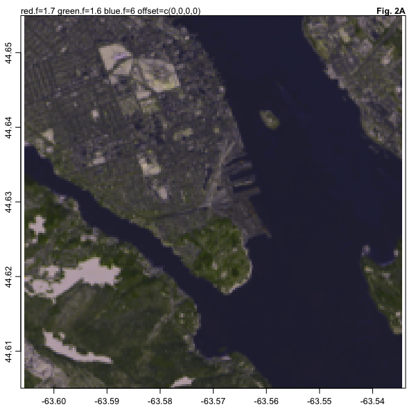
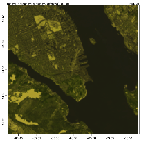
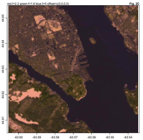
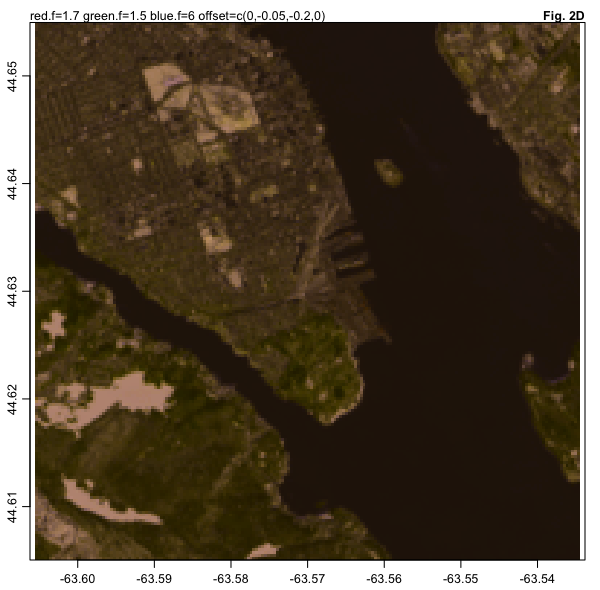
Fig 2A is as in [1] and it has green hues that are natural, and also that permit detection of vegetation in various regions of Halifax that I know to be green in winter. Fig 2B has little to commend it, so it needs no further comment. The snow in Fig 2C is distractingly pink, but in 2D this hue is reduced. Again, the “D” parameters yield reasonably pleasing results.
Now, we apply the same arguments to the Halifax summer scene.
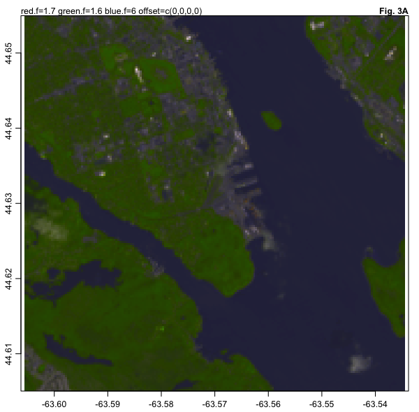
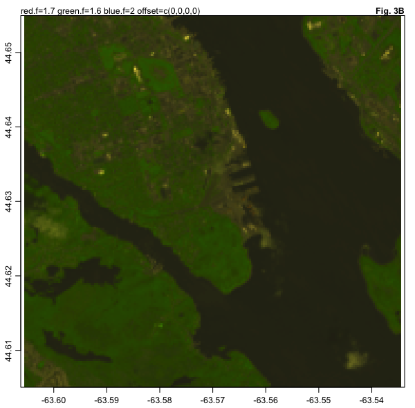
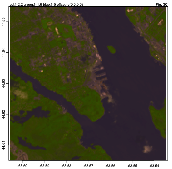
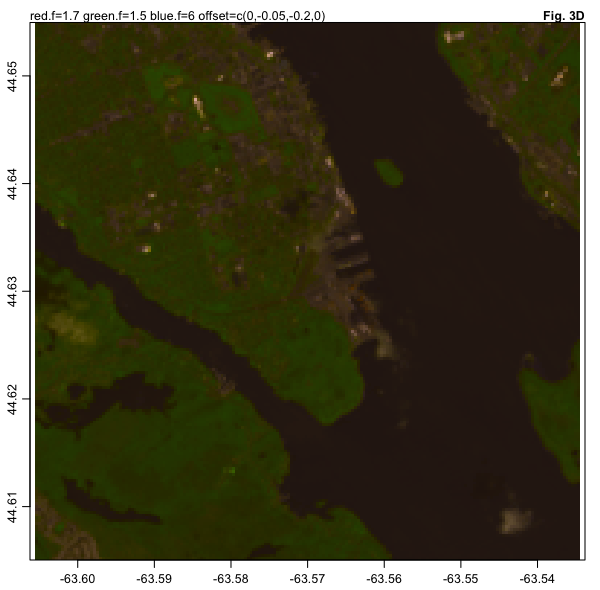
Although 3C and 3D both show the green regions of the city well, the features are perhaps more discernible in 3D.
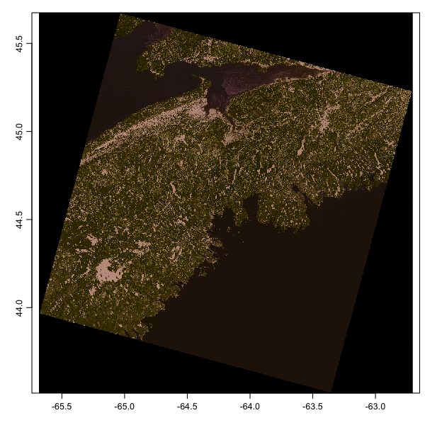
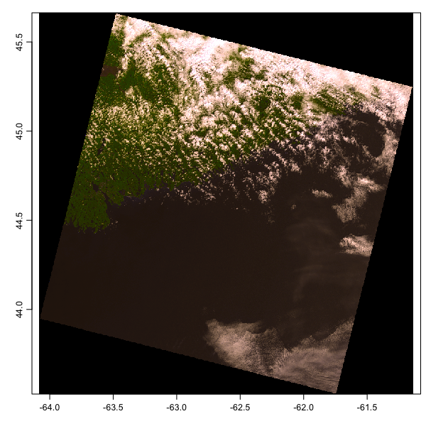
Finally, we test the suggested “D” coefficients with the larger Nova Scotia views, of which the Halifax images were small subregions. Having lived in Nova Scotia my whole life, and flown over it in various seasons, I can say that these colours look reasonably correct over land, in both summer and winter.
1
2
3
4
5
6
7
8
9
10
if (0 == length(ls(pattern="^w$")))
    w <- read.landsat("/data/archive/landsat/LC80080292014065LGN00", band=band)
png("2016-02-21-landsat-winter-ns.png", unit="in", width=6, height=6, res=100, pointsize=9)
plot(w, band="terralook", red.f=1.7, green.f=1.5, blue.f=6, offset=c(0,-0.05,-0.2,0))
dev.off()
if (0 == length(ls(pattern="^s$")))
    s <- read.landsat("/data/archive/landsat/LC80070292014170LGN00", band=band)
png("2016-02-21-landsat-summer-ns.png", unit="in", width=6, height=6, res=100, pointsize=9)
plot(s, band="terralook", red.f=1.7, green.f=1.5, blue.f=6, offset=c(0,-0.05,-0.2,0))
dev.off()
Conclusions
The ‘D’ variants of the figures are all reasonably good, and this suggests new
defaults for plot.landsat(), namely
1
plot.landsat(..., red.f=1.7, blue.f=1.5, green.f=6, offset=c(0,-0.05,-0.2,0), ...)
Even with just three test cases in consideration, it seems clear that these
values are preferable to the old defaults of red.f=2, green.f=2,
blue.f=4, and offset=c(0,0,0,0).
It should be noted that all of these schemes are simply linear transformations, and so cannot be expected to yield the flexibility achieved with nonlinear transformations, as in [1].
Another issue that deserves consideration (perhaps in Part III in this series)
is whether the terralook system is the best for practical purposes. Note that
in [1], the green band of the satellite was used, whereas in terralook, that
band is discarded and instead red, blue, and nir are used for a basis set (see
the help for plot.landsat().)
References and resources
- Article on hand-tuning the colour of a Landsat image, the data for which are also used here in Figure 1 http://earthobservatory.nasa.gov/blogs/elegantfigures/2013/10/22/how-to-make-a-true-color-landsat-8-image/
- Part I of this series https://dankelley.github.io/r/2016/02/20/landsat-hue.html
- Jekyll source code for this blog entry: 2016-02-21-landsat-hue-2.Rmd