Plot an amsr Object

Plot an image of a component of an amsr object.

# S4 method for amsr
plot(
  x,
  y,
  asp = NULL,
  breaks,
  col,
  colormap,
  zlim,
  missingColor = list(land = "papayaWhip", none = "lightGray", bad = "gray", rain =
    "plum", ice = "mediumVioletRed"),
  debug = getOption("oceDebug"),
  ...
)

Arguments

x

an amsr object.

y

character value indicating the name of the band to plot; if not provided, SST is used; see the documentation for the amsr class for a list of bands.

asp

optional numerical value giving the aspect ratio for plot. The default value, NULL, means to use an aspect ratio of 1 for world views, and a value computed from ylim, if the latter is specified in the ... argument.

breaks

optional numeric vector of the z values for breaks in the color scheme. If colormap is provided, it takes precedence over breaks and col.

col

optional argument, either a vector of colors corresponding to the breaks, of length 1 less than the number of breaks, or a function specifying colors. If neither col or colormap is provided, then col defaults to oceColorsTemperature(). If colormap is provided, it takes precedence over breaks and col.

colormap

a specification of the colormap to use, as created with colormap(). If colormap is NULL, which is the default, then a colormap is created to cover the range of data values, using oceColorsTemperature colour scheme. If colormap is provided, it takes precedence over breaks and col. See “Examples” for an example of using the "turbo" colour scheme.

zlim

optional numeric vector of length 2, giving the limits of the plotted quantity. A reasonable default is computed, if this is not given.

missingColor

List of colors for problem cases. The names of the elements in this list must be as in the default, but the colors may be changed to any desired values. These default values work reasonably well for SST images, which are the default image, and which employ a blue-white-red blend of colors, no mixture of which matches the default values in missingColor.

debug

A debugging flag, integer.

...

extra arguments passed to imagep(), e.g. to control the view with xlim (for longitude) and ylim (for latitude).

Details

In addition to fields named directly in the object, such as SSTDay and SSTNight, it is also possible to plot computed fields, such as SST, which combines the day and night fields.

See also

Other things related to amsr data: [[,amsr-method, [[<-,amsr-method, amsr-class, amsr, composite,amsr-method, download.amsr(), read.amsr(), subset,amsr-method, summary,amsr-method

Other functions that plot oce data: download.amsr(), plot,adp-method, plot,adv-method, plot,argo-method, plot,bremen-method, plot,cm-method, plot,coastline-method, plot,ctd-method, plot,gps-method, plot,ladp-method, plot,landsat-method, plot,lisst-method, plot,lobo-method, plot,met-method, plot,odf-method, plot,rsk-method, plot,satellite-method, plot,sealevel-method, plot,section-method, plot,tidem-method, plot,topo-method, plot,windrose-method, plot,xbt-method, plotProfile(), plotScan(), plotTS(), tidem-class

Author

Dan Kelley

Examples

library(oce)
data(coastlineWorld)
data(amsr) # see ?amsr for how to read and composite such objects

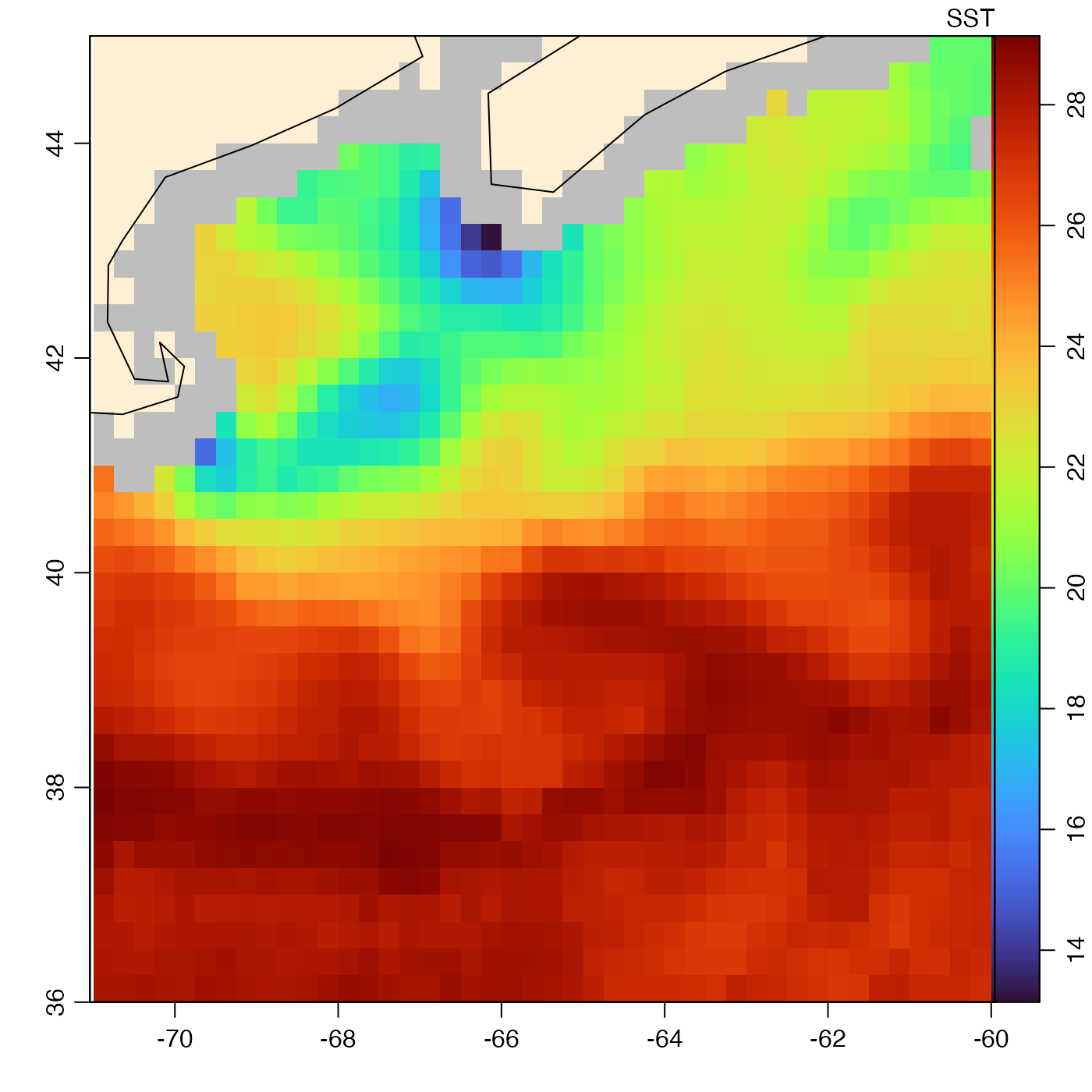
# Example 1: plot with default colour scheme, oceColorsTemperature()
plot(amsr, "SST")
lines(coastlineWorld[['longitude']], coastlineWorld[['latitude']])


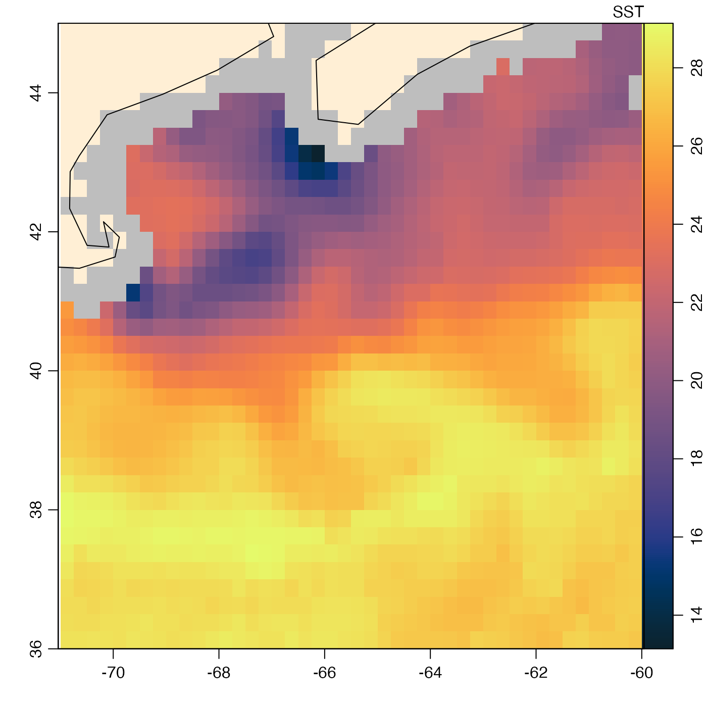# Example 2: 'turbo' colour scheme
plot(amsr, "SST", col=oceColorsTurbo)
lines(coastlineWorld[['longitude']], coastlineWorld[['latitude']])