GMT topography colours (II)
Jan 30, 2014
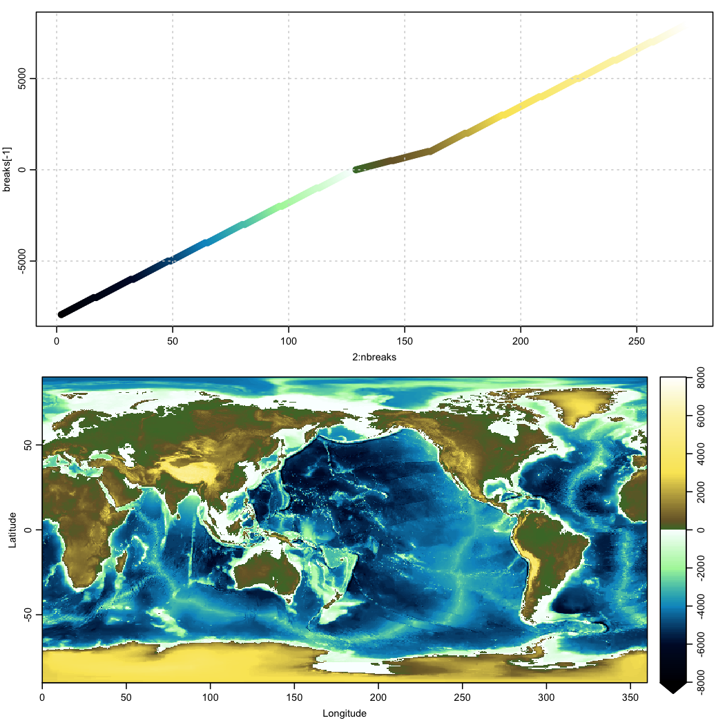
The GMT colour palette is illustrated with ocean topography.
This follows an item about GMT colours. In the meantime I have found a website illustrating the colours, and also the definition files for those palettes.
The palette in question is named GMT_relief, and it is defined in a file that is as follows.
#	$Id: GMT_relief.cpt,v 1.1 2001/09/23 23:11:20 pwessel Exp $
#
# Colortable for whole earth relief used in Wessel topomaps
# Designed by P. Wessel and F. Martinez, SOEST
# COLOR_MODEL = RGB
-8000	0	0	0	-7000	0	5	25
-7000	0	5	25	-6000	0	10	50
-6000	0	10	50	-5000	0	80	125
-5000	0	80	125	-4000	0	150	200
-4000	0	150	200	-3000	86	197	184
-3000	86	197	184	-2000	172	245	168
-2000	172	245	168	-1000	211	250	211
-1000	211	250	211	0	250	255	255
0	70	120	50	500	120	100	50
500	120	100	50	1000	146	126	60
1000	146	126	60	2000	198	178	80
2000	198	178	80	3000	250	230	100
3000	250	230	100	4000	250	234	126
4000	250	234	126	5000	252	238	152
5000	252	238	152	6000	252	243	177
6000	252	243	177	7000	253	249	216
7000	253	249	216	8000	255	255	255
F	255	255	255
B	0	0	0
N	255	255	255
R code to read this file and construct 16-piece linear ramps between the levels is as follows.
1
2
3
4
5
6
7
8
9
10
11
12
13
14
15
16
17
18
19
20
21
22
23
breakPerLevel <- 16 # say
d <- read.table("GMT_relief.cpt", comment="#", nrows=17,
                col.names=c("l", "lr", "lg", "lb",
                            "u", "ur", "ug", "ub"))
nlevel <- length(d$l)
plot(c(1, breakPerLevel), c(1, nlevel))
breaks <- NULL
col <- NULL
for (l in 1:nlevel) {
    lowerColor <- rgb(d$lr[l]/255, d$lg[l]/255, d$lb[l]/255)
    upperColor <- rgb(d$ur[l]/255, d$ug[l]/255, d$ub[l]/255)
    breaks <- c(breaks, seq(d$l[l], d$u[l], length.out=breakPerLevel))
    col <- c(col, colorRampPalette(c(lowerColor, upperColor))(breakPerLevel))
}
## drop a colour to get length matchup for imagep()
col <- col[-1]
nbreaks <- length(breaks)
par(mar=c(3,3,1,1), mgp=c(2,0.7,0), mfrow=c(2,1))
plot(2:nbreaks, breaks[-1], col=col, pch=20, cex=2)
grid()
library(oce)
data(topoWorld)
imagep(topoWorld, breaks=breaks, col=col)
A graph of the results is below.