Introduction

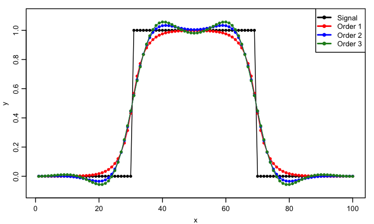
Butterworth filters with order other than 1 have an overshoot phenomenon that can be problematic in some cases. For example, if smoothing is used on an estimate of kinetic energy, overshoots might yield negative values that are nonphysical. This post simply illustrates this with made-up data that the reader can experiment with.

Methods

First, create and plot some fake data, a top-hat function. (Note the use of par to tighten the margins.)

1
2
3
4
5
6
library(signal)
n <- 100
x <- 1:n
y <- ifelse(0.3*n < x & x < 0.7*n, 1, 0)
par(mar=c(3, 3, 1, 1), mgp=c(2, 0.7, 0))
plot(x, y, type='o', pch=20, ylim=c(-0.1, 1.1))

Next, decide on the cutoff frequency for a low-pass filter. Setting W to 0.1 means a cutoff at 1/10-th of the Nyquist frequency.

1
W <- 0.1

Finally, filter with orders 1, 2 and 3, and add coloured lines indicating the results

1
2
3
4
5
6
7
8
9
10
11
12
13
14
15
b1 <- butter(1, W)
y1 <- filtfilt(b1, y)
points(x, y1, type='o', pch=20, col='red')

b2 <- butter(2, W)
y2 <- filtfilt(b2, y)
points(x, y2, type='o', pch=20, col='blue')

b3 <- butter(3, W)
y3 <- filtfilt(b3, y)
points(x, y3, type='o', pch=20, col='forestgreen')

legend("topright", lwd=2, pch=20, 
        col=c("black", "red", "blue", "forestgreen"),
        legend=c("Signal", "Order 1", "Order 2", "Order 3"))

Results

Conclusions

Be careful in using butterworth filters of order 2 and higher, at least in applications that are sensitive to overshoot (e.g. kinetic-energy timeseries).